The debate about the best way to interpret test results is becoming increasingly relevant in the world of conversion rate optimization.
Torn between two inferential statistical methods (Bayesian vs. frequentist), the debate over which is the “best” is fierce. At AB Tasty, we’ve carefully studied both of these approaches and there is only one winner for us.

But first, let’s dive in and explore the logic behind each method and the main differences and advantages that each one offers. In this article, we’ll go over:
[toc]
What is hypothesis testing?
The statistical hypothesis testing framework in digital experimentation can be expressed as two opposite hypotheses:
- H0 states that there is no difference between the treatment and the original, meaning the treatment has no effect on the measured KPI.
- H1 states that there is a difference between the treatment and the original, meaning that the treatment has an effect on the measured KPI.
The goal is to compute indicators that will help you make the decision of whether to keep or discard the treatment (a variation, in the context of AB Tasty) based on the experimental data. We first determine the number of visitors to test, collect the data, and then check whether the variation performed better than the original.

Essentially, there are two approaches to statistical hypothesis testing:
- Frequentist approach: Comparing the data to a model.
- Bayesian approach: Comparing two models (that are built from data).
From the first moment, AB Tasty chose the Bayesian approach for conducting our current reporting and experimentation efforts.
What is the frequentist approach?
In this approach, we will build a model Ma for the original (A) that will give the probability P to see some data Da. It is a function of the data:
Ma(Da) = p
Then we can compute a p-value, Pv, from Ma(Db), which is the probability to see the data measured on variation B if it was produced by the original (A).
Intuitively, if Pv is high, this means that the data measured on B could also have been produced by A (supporting hypothesis H0). On the other hand, if Pv is low, this means that there are very few chances that the data measured on B could have been produced by A (supporting hypothesis H1).
A widely used threshold for Pv is 0.05. This is equivalent to considering that, for the variation to have had an effect, there must be less than a 5% chance that the data measured on B could have been produced by A.
This approach’s main advantage is that you only need to model A. This is interesting because it is the original variation, and the original exists for a longer time than B. So it would make sense to believe you could collect data on A for a long time in order to build an accurate model from this data. Sadly, the KPI we monitor is rarely stationary: Transactions or click rates are highly variable over time, which is why you need to build the model Ma and collect the data on B during the same period to produce a valid comparison. Clearly, this advantage doesn’t apply to a digital experimentation context.
This approach is called frequentist, as it measures how frequently specific data is likely to occur given a known model.
It is important to note that, as we have seen above, this approach does not compare the two processes.
Note: since p-value are not intuitive, they are often changed into probability like this:
p = 1-Pvalue
And wrongly presented as the probability that H1 is true (meaning a difference between A & B exists). In fact, it is the probability that the data collected on B was not produced by process A.
What is the Bayesian approach (used at AB Tasty)?
In this approach, we will build two models, Ma and Mb (one for each variation), and compare them. These models, which are built from experimental data, produce random samples corresponding to each process, A and B. We use these models to produce samples of possible rates and compute the difference between these rates in order to estimate the distribution of the difference between the two processes.
Contrary to the first approach, this one does compare two models. It is referred to as the Bayesian approach or method.
Now, we need to build a model for A and B.
Clicks can be represented as binomial distributions, whose parameters are the number of tries and a success rate. In the digital experimentation field, the number of tries is the number of visitors and the success rate is the click or transaction rate. In this case, it is important to note that the rates we are dealing with are only estimates on a limited number of visitors. To model this limited accuracy, we use beta distributions (which are the conjugate prior of binomial distributions).
These distributions model the likelihood of a success rate measured on a limited number of trials.
Let’s take an example:
- 1,000 visitors on A with 100 success
- 1,000 visitors on B with 130 success
We build the model Ma = beta(1+success_a,1+failures_a) where success_a = 100 & failures_a = visitors_a – success_a =900.
You may have noticed a +1 for success and failure parameters. This comes from what is called a “prior” in Bayesian analysis. A prior is something you know before the experiment; for example, something derived from another (previous) experiment. In digital experimentation, however, it is well documented that click rates are not stationary and may change depending on the time of the day or the season. As a consequence, this is not something we can use in practice; and the corresponding prior setting, +1, is simply a flat (or non-informative) prior, as you have no previous usable experiment data to draw from.
For the three following graphs, the horizontal axis is the click rate while the vertical axis is the likelihood of that rate knowing that we had an experiment with 100 successes in 1,000 trials.
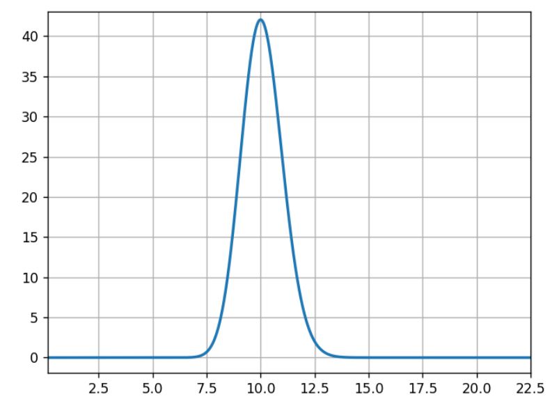
What usually occurs here is that 10% is the most likely, 5% or 15% are very unlikely, and 11% is half as likely as 10%.
The model Mb is built the same way with data from experiment B:
Mb= beta(1+100,1+870)
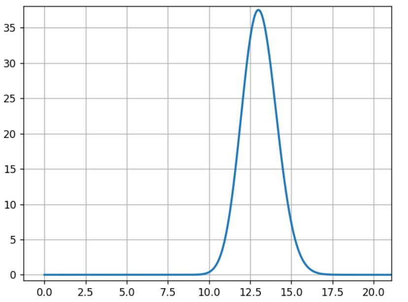
For B, the most likely rate is 13%, and the width of the curve’s shape is close to the previous curve.
Then we compare A and B rate distributions.
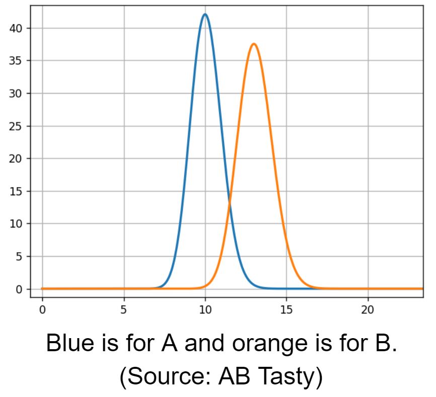
We see an overlapping area, 12% conversion rate, where both models have the same likelihood. To estimate the overlapping region, we need to sample from both models to compare them.
We draw samples from distribution A and B:
- s_a[i] is the i th sample from A
- s_b[i] is the i th sample from B
Then we apply a comparison function to these samples:
- the relative gain: g[i] =100* (s_b[i] – s_a[i])/s_a[i] for all i.
It is the difference between the possible rates for A and B, relative to A (multiplied by 100 for readability in %).
We can now analyze the samples g[i] with a histogram:
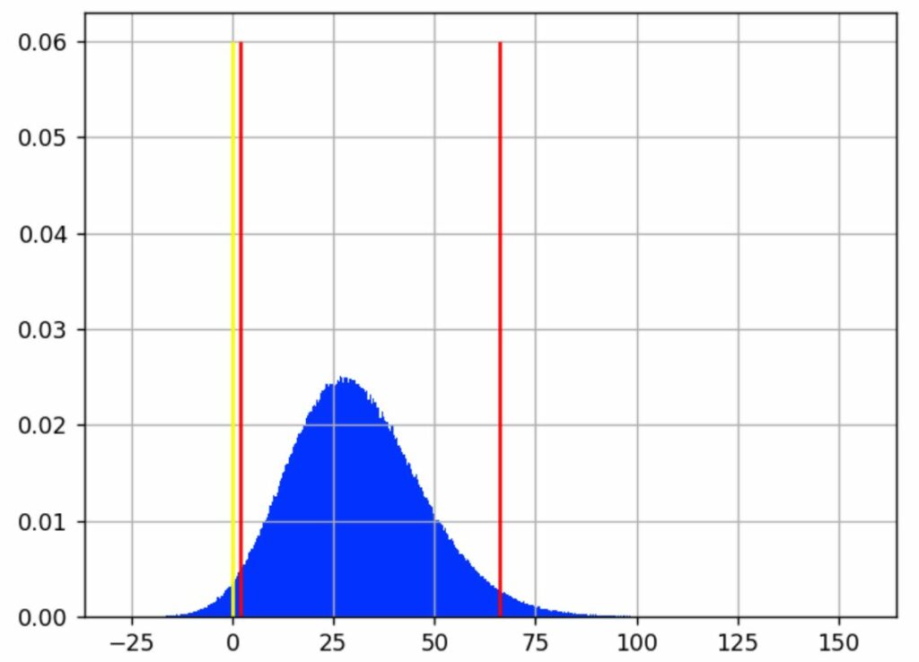
We see that the most likely value for the gain is around 30%.
The yellow line shows where the gain is 0, meaning no difference between A and B. Samples that are below this line correspond to cases where A > B, samples on the other side are cases where A < B.
We then define the gain probability as:
GP = (number of samples > 0) / total number of samples
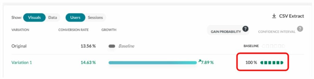
With 1,000,000 (10^6) samples for g, we have 982,296 samples that are >0, making B>A ~98% probable.
We call this the “chances to win” or the “gain probability” (the probability that you will win something).
The gain probability is shown here (see the red rectangle) in the report:
Using the same sampling method, we can compute classic analysis metrics like the mean, the median, percentiles, etc.
Looking back at the previous chart, the vertical red lines indicate where most of the blue area is, intuitively which gain values are the most likely.
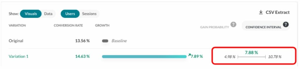
We have chosen to expose a best- and worst-case scenario with a 95% confidence interval. It excludes 2.5% of extreme best and worst cases, leaving out a total of 5% of what we consider rare events. This interval is delimited by the red lines on the graph. We consider that the real gain (as if we had an infinite number of visitors to measure it) lies somewhere in this interval 95% of the time.
In our example, this interval is [1.80%; 29.79%; 66.15%], meaning that it is quite unlikely that the real gain is below 1.8 %, and it is also quite unlikely that the gain is more than 66.15%. And there is an equal chance that the real rate is above or under the median, 29.79%.
The confidence interval is shown here (in the red rectangle) in the report (on another experiment):
What are “priors” for the Bayesian approach?
Bayesian frameworks use the term “prior” to refer to the information you have before the experiment. For instance, a common piece of knowledge tells us that e-commerce transaction rate is mostly under 10%.
It would have been very interesting to incorporate this, but these assumptions are hard to make in practice due to the seasonality of data having a huge impact on click rates. In fact, it is the main reason why we do data collection on A and B at the same time. Most of the time, we already have data from A before the experiment, but we know that click rates change over time, so we need to collect click rates at the same time on all variations for a valid comparison.
It follows that we have to use a flat prior, meaning that the only thing we know before the experiment is that rates are in [0%, 100%], and that we have no idea what the gain might be. This is the same assumption as the frequentist approach, even if it is not formulated.
Challenges in statistics testing
As with any testing approach, the goal is to eliminate errors. There are two types of errors that you should avoid:
- False positive (FP): When you pick a winning variation that is not actually the best-performing variation.
- False negative (FN): When you miss a winner. Either you declare no winner or declare the wrong winner at the end of the experiment.
Performance on both these measures depends on the threshold used (p-value or gain probability), which depends, in turn, on the context of the experiment. It’s up to the user to decide.
Another important parameter is the number of visitors used in the experiment, since this has a strong impact on the false negative errors.
From a business perspective, the false negative is an opportunity missed. Mitigating false negative errors is all about the size of the population allocated to the test: basically, throwing more visitors at the problem.
The main problem then is false positives, which mainly occur in two situations:
- Very early in the experiment: Before reaching the targeted sample size, when the gain probability goes higher than 95%. Some users can be too impatient and draw conclusions too quickly without enough data; the same occurs with false positives.
- Late in the experiment: When the targeted sample size is reached, but no significant winner is found. Some users believe in their hypothesis too much and want to give it another chance.
Both of these problems can be eliminated by strictly respecting the testing protocol: Setting a test period with a sample size calculator and sticking with it.
At AB Tasty, we provide a visual checkmark called “readiness” that tells you whether you respect the protocol (a period that lasts a minimum of 2 weeks and has at least 5,000 visitors). Any decision outside these guidelines should respect the rules outlined in the next section to limit the risk of false positive results.
This screenshot shows how the user is informed as to whether they can take action.
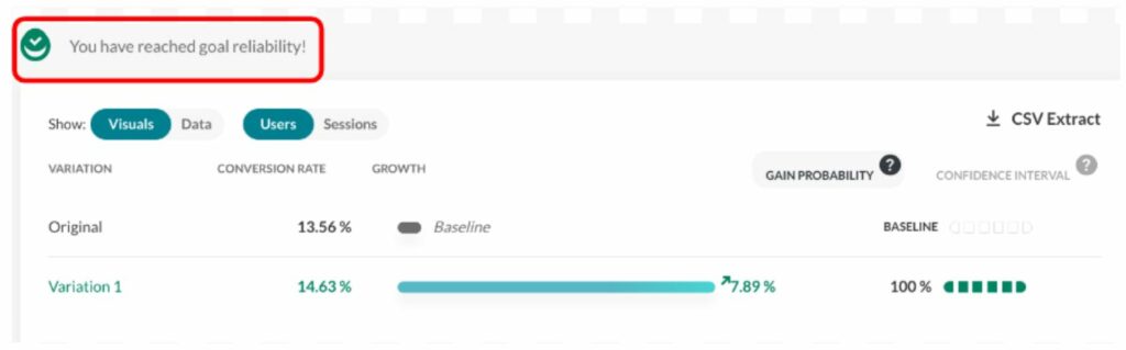
Looking at the report during the data collection period (without the “reliability” checkmark) should be limited to checking that the collection is correct and to check for extreme cases that require emergency action, but not for a business decision.
When should you finalize your experiment?
Early stopping
“Early stopping” is when a user wants to stop a test before reaching the allocated number of visitors.
A user should wait for the campaign to reach at least 1,000 visitors and only stop if a very big loss is observed.
If a user wants to stop early for a supposed winner, they should wait at least two weeks, and only use full weeks of data. This tactic is interesting if and when the business cost of a false positive is okay, since it is more likely that the performance of the supposed winner would be close to the original, rather than a loss.
Again, if this risk is acceptable from a business strategy perspective, then this tactic makes sense.
If a user sees a winner (with a high gain probability) at the beginning of a test, they should ensure a margin for the worst-case scenario. A lower bound on the gain that is near or below 0% has the potential to evolve and end up below or far below zero by the end of a test, undermining the perceived high gain probability at its beginning. Avoiding stopping early with a low left confidence bound will help rule out false positives at the beginning of a test.
For instance, a situation with a gain probability of 95% and a confidence interval like [-5.16%; 36.48%; 98.02%] is a characteristic of early stopping. The gain probability is above the accepted standard, so one might be willing to push 100% of the traffic to the winning variation. However, the worst-case scenario (-5.16%) is relatively far below 0%. This indicates a possible false positive — and, at any rate, is a risky bet with a worst scenario that loses 5% of conversions. It is better to wait until the lower bound of the confidence interval is at least >0%, and a little margin on top would be even safer.
Late stopping
“Late stopping” is when, at the end of a test, without finding a significant winner, a user decides to let the test run longer than planned. Their hypothesis is that the gain is smaller than expected and needs more visitors to reach significance.
When deciding whether to extend the life of a test, not following the protocol, one should consider the confidence interval more than the gain probability.
If the user wants to test longer than planned, we advise to only extend very promising tests. This means having a high best-scenario value (the right bound of the gain confidence interval should be high).
For instance, this scenario: gain probability at 99% and confidence interval at [0.42 %; 3.91%] is typical of a test that shouldn’t be extended past its planned duration: A great gain probability, but not a high best-case scenario (only 3.91%).
Consider that with more samples, the confidence interval will shrink. This means that if there is indeed a winner at the end, its best-case scenario will probably be smaller than 3.91%. So is it really worth it? Our advice is to go back to the sample size calculator and see how many visitors will be needed to achieve such accuracy.
Note: These numerical examples come from a simulation of A/A tests, selecting the failed ones.
Confidence intervals are the solution
Using the confidence interval instead of only looking at the gain probability will strongly help improve decision-making. Not to mention that even outside of the problem of false positives, it’s important for the business. All variations need to meet the cost of its implementation in production. One should keep in mind that the original is already there and has no additional cost, so there is always an implicit and practical bias toward the original.
Any optimization strategy should have a minimal threshold on the size of the gain.
Another type of problem may arise when testing more than two variations, known as the multiple comparison problem. In this case, a Holm-Bonferroni correction is applied.
Why AB Tasty chose the Bayesian approach
Wrapping up, which is better: the Bayesian vs. frequentist method?
As we’ve seen in the article, both are perfectly sound statistical methods. AB Tasty chose the Bayesian statistical model for the following reasons:
- Using a probability index that corresponds better to what the users think, and not a p-value or a disguised one;
- Providing confidence intervals for more informed business decisions (not all winners are really interesting to push in production.). It’s also a means to mitigate false positive errors.
At the end of the day, it makes sense that the frequentist method was originally adopted by so many companies when it first came into play. After all, it’s an off-the-shelf solution that’s easy to code and can be easily found in any statistics library (this is a particularly relevant benefit, seeing as how most developers aren’t statisticians).
Nonetheless, even though it was a great resource when it was introduced into the experimentation field, there are better options now — namely, the Bayesian method. It all boils down to what each option offers you: While the frequentist method shows whether there’s a difference between A and B, the Bayesian one actually takes this a step further by calculating what the difference is.
To sum up, when you’re conducting an experiment, you already have the values for A and B. Now, you’re looking to find what you will gain if you change from A to B, something which is best answered by a Bayesian test.


 Chad Sanderson (Convoy)
 Jonny Longden (Journey Further)